Statistics

There’re convenience functions for entering data, obtaining statistical metrics, and graphing statistical data. These functions are located in the Stat and graph (via key ∿ (PLOT)) menus.

You may also import data from your computer, after getting set up, as explained here.

Statistical data is contained in a special variable, named ∑DAT, in the current folder. In order to work on various projects, each with their own set of statistical data, just create a folder for each project.

In this tutorial, you will exercise some basic statistics using fictive example data.

Let’s start by creating a folder for our project.

Tap My Data, and make sure the top-level is showing.

Tap the “+” to get the “Add Category” (folder) dialog, type My Stats in the text field, and tap Save.

If you had statistical data to import you would now proceed into the Sharing dialog and download.

For now on, we shall just enter some data.

Switch back to ND1 or ND1 (Classic).

Tap the database key (⊛ (USER)) twice and step into the My Stats folder. It will be empty.

Clear the stack. (⌧ (CLEAR))

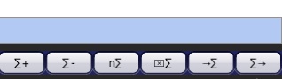
Switch to the statistics menu: Tap the Menu key, tap Stat.

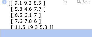
The following shall be our statistical data to be entered:

CI PI JR

9.1 9.2 8.5

5.8 4.6 7.7

6.5 6.1 7.0

7.6 7.8 6.0

11.5 19.3 5.8

We’ll type in row by row as a vector and use the ∑+ key to add each row to the current statistics matrix, ∑DAT in the current folder. (Which doesn’t yet exist,)

Enter [9.1,9.2,8.5

Tap ∑+

At this point, the ∑DAT variable has been created, and the matrix populated with the first row of data.

Type (but don’t enter) [5.8,4.6,7.7

Tap ∑+

You don’t have to use Enter to a row, and can save a keystroke.

Let’s make a typo on the next row:

Type [6.5,6.1,5

Tap ∑+

Let’s say at this point you noticed the typo.

Tap ∑-

∑- pulls the last row out of the current statistics matrix and displays it on the stack.

Tap ⇩ (EDIT) to edit this row. (Modern: ⇩ is the 2nd level function of the Expresssion/Name key, not Drop.)

Tap ⌫ (←) twice, tap “7” to correct the row, and tap ∑+ to add the corrected row to the statistics matrix.

In this fashion, add the last two rows:

Type [7.6,7.8,6, tap ∑+

Type [11.5,19.3,5.8, tap ∑+

Tap ∑→ (RCL∑)

This recalled the statistics matrix. You can now check there’re no typos. Edit the matrix, if there’s one.

Drop it off the stack with ⇓ (DROP).

Now, various keys in the menu will give you statistical metrics for the data you entered.

Let’s try a few.

Tap n∑

This simply tells us you how many rows you have.

(Classic: tap → (NEXT) to go to the next menu page)

Tap total (TOT)

This gives you the total sum for each column.

Tap mean (MEAN)

This gives you the average for each column.

Tap stddev (SDEV)

This is the standard deviation for each column.

In order to see this formatted more nicely, switch to the mode menu and switch to 2 fixed digits after the point:

Tap ⌽ (MODE), tap “2”, tap fix (FIX)

There’re various functions that work on column pairs.

Let’s assume you’re interested to see if there’s a correlation between the first two columns of your data.

Go back to the Stat menu.

Tap → (NEXT) until you see corr (CORR).

Tap corr (CORR)

1.0 would indicate an entirely linear dependency. 0.96 indicates there is indeed an almost linear correlation between those columns.

Cov (COV) can show you the covariance between columns.

Now, we entered three columns. Which columns do these functions operate on?

By default, that’s columns number 1 and 2. But you can change that with the ∑cols (COL∑) function.

To see if there’s a correlation between 1 and 3, do this:

Enter 1

Enter 3

Tap ∑cols (COL∑). This establishes a new column pairing.

Tap corr (CORR)

No, they aren’t correlated. (If anything, there’s a weak negative correlation between them.)

Let’s go back to associating columns 1 and 2:

Type “1,2” (w/o quotes), tap ∑cols (COL∑).

Since these columns were highly correlated, let’s do a linear regression to obtain the slope and y-offset of the best-fit line through the data in columns 1 and 2.

Tap linear (LR)

The slope of the regression line is 2.45, it’s y-offset (intersection with the y-axis) is at -10.43.

These results are also stored in a special variable, ∑PAR, in the current folder. (That variable is a vector, and it also holds the indices of the associated columns.)

Once a linear regression has been performed, values can be predicted. (The higher the correlation, the higher the confidence you can place in any prediction.)

Let’s predict the value for the second column, for a new value of 6 for the first:

Tap “6”

Tap predict (PREDV)

Hence, PI is predicted to be 4.26 when CI is 6.

Let’s turn off fixed number display, as we no longer need it: Once more, go to the Mode menu and tap std (STD).

You may also want to clear the stack. (⌧ (CLEAR))

Now, let’s assume we want to tag our rows with some year descriptors and produce a graph of the annotated data.

Go back to the Stat menu.

We need a new column, but ∑+ only adds rows. We can employ a little trick to accomplish our goal.

First, let’s type in the data for our new column:

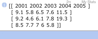
Enter 2001,2002,2003,2004,2005

Tap ∑→ (RCL∑)

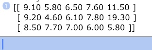
Now, let’s transpose the matrix to change rows into columns, and vice versa.

We can go to the Array menu, and tap the trans (TRN) soft-key there.

If we’re too lazy for that, we can just type in the correct ND1 or ND1 Classic function name, on the edit line:

Type “transpose” (w/o quotes) or “TRN” (w/o quotes) (both names will work in either mode)

and enter.

Let’s dissolve the matrix, so we can add the new data to it.

Once again, we could use the right soft-key (array→ (ARRY→)) in the Array menu for that, or type the function.

Type “toElements” (w/o quotes)

and enter.

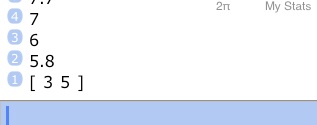
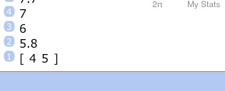
(this function places all matrix elements on the stack, as well as a size vector. [3 5] tells us this is (or, rather, was) a 3x5 matrix)

Now, we do know our five new numbers are on top of the dissolved elements on the stack.

Let’s change the matrix dimensions to include them, and recreate a matrix from stack contents:

Tap ⇩ (EDIT) to edit the vector, and change it into [4,5]

or (perhaps easier) enter [1,0] and type “+”.

With your stack now looking like this

type “fromElements” (w/o quotes)

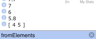
and enter.

Let’s transpose this to restore our old row, column order:

Type transpose

and enter

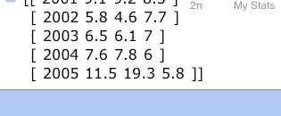
(notice the new data as first column)

and save the result as our new statistics matrix:

Tap →∑ (STO∑)

Now, we had to go through a couple of hoops to accomplish our goal. Had we been happy to just append our new data it would have been easier: we would have entered the data as a vector, transposed the statistics matrix, saved it, used ∑+ to add our new vector, recalled the matrix, transposed and saved it.

Once you know what to do, you can perform steps like this quite quickly.

Anyway. We’re ready to graph.

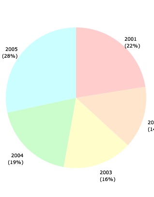
Go to the graph menu (∿ (PLOT)), advance through the menu pages until you see pie∑.

Tap pie∑

Double-tap to see it in full glory:

Double-tap, to come back to stack display, and tap the Space key to quit graphics display.