Specifications            Quick Tour            Tutorials            Reference            Forums

ND1 tries to make it easy for you to get the math in your head into your calculator.

There’re no less than 5 ways to program ND1. These leverage two programming environments: RPL and JavaScript. You used one in the Quick Tour, when you recorded your actions and ended up with an RPL program.

We assume here that you completed the Quick Tour and Just a Few More Things. If not, please backtrack and come back later.

This tutorial gives you an overview of the five programming methods, and is meant to give you a good idea of how you can go about writing your own functions, and which method(s) to use.

Every introduction to programming obligatorily starts with a program called “Hello World”. We’ll not fight it.

Here’s you doing Hello World in RPL: (this time without time pressure)

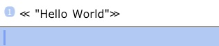
Every RPL program starts with this special character: ≪

You find it as a 2nd level function over the Space key (bottom left of the keypad).

Tap 2nd level and ≪

Tap the edit line.

Get a double quote from the standard keyboard and type: “Hello World

Stop there. Do not enter a closing double-quote. (You can always let ND1 close off for you.)

Enter.

You’re done.

Tap Eval.

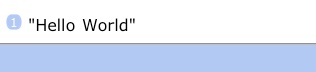
This is not a spectacular result, but, believe it or not, this is a program, and you just ran it (when you tapped Eval).

Undo. (You know how to do that, right? Just press the ↩ key.)

Actually, let’s save your program (which should now be back on level 1).

Make sure My Vars is the current folder; if not, navigate there. (You know how to do that, too, right? If not, back to the tour!)

Store it under ‘Hello’. (Enter ‘Hello and tap →⊛ (STO))

Make sure you see My Var entries.

Now press the new Hello key. That’s a bit more impressive, but looks as if you just recalled a fixed text string. (Which you didn’t. You ran a program which happened to push a string on the stack.)

For completeness, let’s do the same in JavaScript. Let’s use the multi-line editor this time.

Double-tap the edit line to expand it, and then enter the following

Enter that, type HelloJS, and tap →⊛ (STO) to store this program under HelloJS.

Run that program by tapping the HelloJS soft-key.

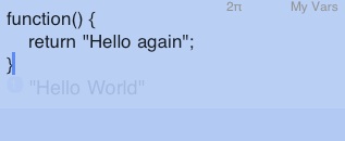
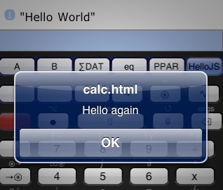
Let’s make a simple edit to this function.

Edit HelloJS by tapping the 2nd level key and the HelloJS soft-key.

This will recall the contents of HelloJS in the multi-line editor.

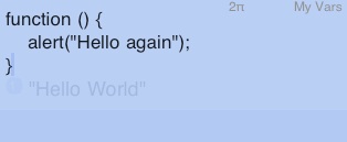
Edit the program text to read:

Enter that, tap ‘ (single quote), tap the HelloJS soft-key, and tap →⊛ (STO)

Now run that program.

This was a minimal exploration of programming methods #3 (RPL Program) and #1 (JavaScript).

Let’s look at user functions that do some actual work.

Switch back to ND1, navigate to Project X.

Enter 5 and 4.

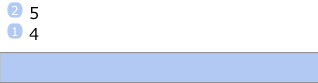
Find and press the dist soft-key.

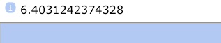
This computes the square root of the sum of squares of the input arguments, 4 and 5.

There’re more distXXX functions, and they all do the same. Each one is using a different programming method.

Here’s the “source code” for each function:

dist:                f(x, y) = sqrt(x*x + y*y)                                    “natural math entry”

distance:        function(x, y) { return sqrt(x*x + y*y); }            JavaScript

dist_rpl:          ≪ → x y ≪ x SQ y SQ + sqrt ≫ ≫                    RPL (using local variables)

dist_rpl_func: ≪ → x y 'sqrt(x*x + y*y)' ≫                               “RPL user function”

Stack-action-recording aside, “natural math entry” is arguably the easiest way to write a user function, as it looks just like math. ND1 changes these functions into JavaScript. It’s used for short functions that return one result.

“RPL user functions” combine RPL with expressions and are also limited to returning one result.

There’s also RPL+, which is a superset of RPL, with extensions unique to MorphEngine, ND1’s calculator engine.

There’re more ways to write this function. Here’re alternatives in RPL and RPL+:

dist_rpl2:        ≪ SQ SWAP SQ + √ ≫                                  RPL (using only the stack)

dist_rpl+:        ≪ =x =y √(x^2+y^2) ≫                                    RPL+ (using “immediate algebraic expression”)

Here’s a look at another example.

Let’s imagine ND1 had no function to randomize a matrix, and you needed one.

Let’s say the function’s job shall be to take an existing matrix and replace all its elements with random numbers from -9 to 9. (This happens to be what the built-in function RANM does. Here’s telling you that, for a change, *before* you start the job...)

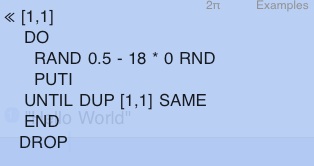
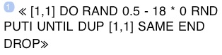
Here’s how you could do this in RPL (old-school):

Tap the 2nd level key and ≪ to start an RPL program.

Double-tap the edit line to go multi-line, and enter the following program:

You may wish to use soft-keys from the Program, Real, Array, and Stack menus to help with entering this text:

Program: [], DO, UNTIL, END, SAME

Real: RAND, RND

Array: PUTI

Stack: DROP

Enter. (If your calculator is in expanded key mode, and you see no Enter key, shake the device to shrink the keypad and get back the line of keys which contains the Enter key.)

This program

- Pushes a vector [1,1] onto the stack; this is going to be used as the index to the first column in the first row of our matrix

1. -Uses a do-until construct, which performs
   

2. -a RAND call; which produces a random number from 0 to 1
   

3. -subtracts 0.5 from it, mapping it to -0.5 to 0.5
   

4. -multiplies by 18, mapping it to -9 to 9
   

5. -calls 0 RND, which rounds the number to an integer
   

6. -calls PUTI
   

  PUTI is a convenient functions; as documented in the reference (along with all the other functions we using here right now), it expects a matrix and an index vector and a value on the stack, places the value at the indexed location, and returns the matrix again, together with an updated index vector that points to the next position.

  After our first run through, then, a random number will have been placed at position 1,1 in the matrix, and the matrix and a index vector [2,1] (pointing to the next location in the matrix) will be on the stack again.

1. -a UNTIL call, which is part of the do-until structure; it executes instructions until the next END, then checks if the first value on the stack is non-zero (or “true”). If not, it jumps back to its DO for another “loop” through the instructions. If yes, it jumps until after the END, and continues instructions there.
   

  Now, [1,1], a comparison value, is pushed on the stack and SAME is called. SAME compares two values and says “true” if there’re the same, otherwise “false”.

On the first loop, we said our index vector will have been updated to [2,1] so the comparison result will be “false”, and another loop will be made.

A new random number will be placed in the matrix at position [2,1], the index updated to [3,1], etc.

When the last element of the matrix will have been reached, say, [5,5] for a 5x5 matrix, the index returned by PUTI will be wrapped to the beginning and become [1,1]. At this point our UNTIL condition is “true” and the program continues past END.

All that’s left to do there is a DROP (of the [1,1] index vector).

What’s left on the stack, will be a random matrix.

Let’s try it out.

First save your program under ‘RNDM’.  (Enter ‘RNDM, tap →⊛ (STO))

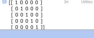
Now, create a 5x5 matrix, by

entering 5

switching to the Array menu, finding the identity (IDN) soft-key and tapping it.

(The is a case where typing (“5,IDN” (w/o quotes)) would have been quicker.)

Now switch the menu back to My Vars by tapping the ⊛ (USER) key, and tap RNDM.

This is what you should see

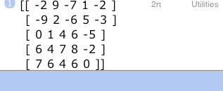
Except, your values will be different. After all, this is a *random* matrix.

Now, this wasn’t too bad. But also not that great.

For something much faster, you can accomplish the same in JavaScript.

When programming in JavaScript you have quite a few options in ND1. You can write in pure JavaScript with no knowledge of the MorphEngine API. Or, you can write “against” that API. (Meaning, you use the API.)

Here’s the JavaScript code, that will accomplish the same goal, using the same technique.

You may enter it on the multi-line edit line:

function(m) {

    for (i=0; i<m.length; i++)

        for (j=0; j<m.length; j++)

            m[i][j] = round((random()-0.5)*18, 0);

    return m;

}

Store your JavaScript function as ‘randM’.

Now run it on the matrix you still have on the stack. This version of the code can easily run on a matrix that’s 100x100 or even 500x500 elements (that’s 250,000 elements!) large. It will randomize that 500x500 matrix in just two seconds. (On an iPhone 3GS.)

Finally, here’s what array processing can do for you:

≪ [ [randomize 0.5 - 18 * 0 RND] MAP] MAP ≫

This code doesn’t run as fast as the JavaScript code, but it’s fast (much faster than the traditional RPL code above).

And, again, it’s easier to write and read.

Here’s another, even shorter version, using the “map” function:

≪ [ randomize 0.5 - 18 * 0 RND ] map ≫

The exact function accomplished by all these programs is available in the calculator through the built-in function RANM (a Classic function). If you wish to randomize a matrix to values between 0 and 1, you need no program either: just issue the randomize command.

Hopefully, this has given you a (good) taste of how programming of user functions for ND1 looks like.

If you’re ready for more, do the FibTriangle tutorial, which dives a bit deeper and shows–using a math exploration we consider fun–how you can mix JavaScript and RPL (give-away: there’s nothing to it; it’s automatic).

Also, there’re many downloadable coding examples available. You can find them under My Data | Downloadables | Shared Folders, which are discussed in the Shared Data section of the forums. RNDM and randM are in the Examples downloadable folder. Project Euler, again, has great, short examples, and is highly recommended.

Writing user functions, in RPL or JavaScript, is one of the ways you can extend ND1, but there’re others.

Using JavaScript, you can

1. -alter or extend built-in functions
   

2. -“inject” your own functions permanently into ND1 (and make them available outside of the current folder),
   

3. -write your own data types,
   

4. -or extensions that do things completely different from calculation-related functionality.
   

These options are explored in depth in various chapters in the Reference section.

There’s no one best language to use.

Here’re some guidelines:

1. -if you never programmed before, learn and use RPL+ (and skip to the next section now)
   

1. -if you’re used to HP’s RPL, use that, and learn RPL+ to broaden what you can do, and how easily you can do it
   

2. -if you’re looking for all-out speed, use JavaScript or RPL+ with array processing (see below)
   

3. -if you know JavaScript, use that, but also learn RPL+. You can pick it up in no time, and it’s far more convenient for smaller programs, and those that rely on data types, not native to JavaScript, such as BigInts. Array processing in RPL+ makes for very concise and readable programs, that run at almost JavaScript speed
   

4. -if you want to extend or overwrite built-in functions or create new data types, use JavaScript
   

5. -if you want to do graphics programming using the HTML5 Canvas, use JavaScript; for data plotting needs you may be served by the built-in functions and those from the Plot downloadable folder
   

If you know C or Java or another C-like languages, know that JavaScript is C-like too. For the kind of programs you write on this calculator, you need to know nothing about “client-side” (web-style) JavaScript. C code can often be used almost verbatim, after changing all type declarations (int, char, etc.) into “var”. What helps knowing is the command-set of the calculator.

RPL+ is a modernized version of RPL. Its a simple, yet strong language, for writing short programs that deal with the kind of data (numbers (real, complex, big), vectors, matrices, etc.) that this calculator supports. For math tasks, 10 lines of RPL+ can often do, what you’d need 100+ lines of C code for, or 30 lines of C code using a math library.

Let’s jump back into writing some code. Switch back to the My Vars folder.

The calculator can convert from °F to °C.

For example, to convert 68 °F, you’d

Enter 68

Enter '˚F

Enter '˚C

and tap convert (CONVERT) from the keypad (using the 2nd-level key).

You will now see

20

'˚C'

on the stack, which is your answer.

The degree symbol is found as a soft-key in the String menu. It’s also atop the 1 key in Classic mode. If you don’t want to hunt for it, you may instead type ‘Fahrenheit’ and ‘Celsius’.

Now, let’s assume you have to do this conversion often, and you’d like a program that

1. -takes as input a number representing degrees Fahrenheit
   

2. -does the conversion
   

3. -drops the ‘°C’ (or ‘Celsius’, if that’s what you’re using) from the result
   

Enter ≪ 'Fahrenheit' 'Celsius' CONVERT DROP

Enter FtoC

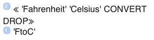
Tap →⊛ (STO)

Your program is done and stored in a variable FtoC in My Vars now. You may have to use the → (NEXT) key to go to the last page of My Vars to see your new variable.

Now try out your program.

Enter 68

Tap the FtoC soft-key

You should see the result, 20, displayed. We intentionally dropped the Celsius denotation with the DROP command.

This is a simple program representative of a routine that wraps a calculator function to make it more suitable for your daily use. The program is identical to the steps you would perform with key-presses on the calculator. In fact, you could have recorded this program by using the record and stop functions from the Program menu (just like you did in the Quick Tour).

Note: there’s no code required to tell RPL what your input argument to a function is. Inside our function, we’re using CONVERT, a function that expects three input arguments, and our program provides two of them. The “missing” input comes from the stack. That is, it’s going to be the number you enter before running the program.

This is a strength, and an important to thing to know about RPL: an RPL program does not need to provide its own inputs or declare them in any way. It will interact with the stack and both get inputs from the stack and put outputs to the stack. Without added programming structures that change the flow of instructions in a program (we’re coming to that in a minute), an RPL program is simply like a recording of steps performed with the calculator.

You’re now ready to understand this program

≪ SQ SWAP SQ + √ ≫

which was the alternative (and most concise) RPL implementation for the distance function √(x^2+y^2).

With two numbers on the stack, 5 and 4, the program will square the second, then swap both numbers, square the first, add them, and apply the square root function. That last value remains on the stack and represents the programs output.

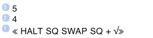
Oftentimes, it’s very helpful to “see” a program perform, as it does its work step-by-step. There’s an instruction that you can insert anywhere in your program, to make it stop and switch to single-stepping and display a dialog that shows you what it does, step-by-step: HALT

Enter 5

Enter 4

Enter ≪ HALT SQ SWAP SQ + √            (you will have to dismiss the iOS keyboard to type “√”, or type sqrt instead)

You could store this program under a name now, but you don’t have to.

With RPL, you can run a program on position 1 of the stack by tapping the Eval key.

Do that now.

You will see the following dialog:

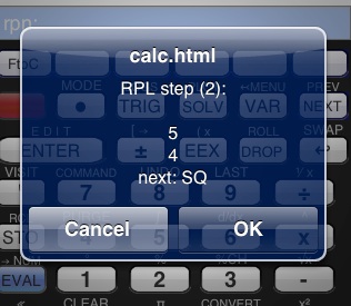
This is the RPL debugger.

It’ll tell you:

1. -the number of the program step you’re at
   

2. -the contents of the first three stack positions
   

3. -what operation comes next
   

Here it shows that

1. -5 and 4 are on the stack
   

2. -next up is the SQ instruction
   

Cancel kills program execution.

OK proceeds to the next step.

Tap OK to proceed.

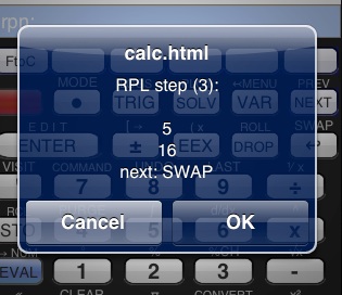
You now see the effect that SQ had on the stack:

it changed 4 into 16, as you’d expect from a “square” function

Keep stepping through your program, until, at last, the dialog is dismissed and you see the result:

If you cancel the debugger dialog, the program will stop execution and your stack will reflect the state of a program having run its course only part-way. You’ll usually want to tap ↩ (Undo) then.

Press ↩ (Undo) now, to get your program code back.

If the program executed properly, edit it to remove the HALT command, and store it under a name of your liking.

If a program needs adjustment (forgotten command, or suchlike), you’d edit and run it repeatedly, until it performs properly. You can do this with or without using the HALT command. The point is, you don’t have to store an RPL program after every edit. Since you can execute an unnamed program on the stack, you can postpone the storing step until you’re done “debugging” the program.

Let’s write a program to find all primes below a given number. We’re going to use the built-in function isPrime (ISPRIME?) to assist us in this task.

The program is to

1. -assume 100 as upper limit for our search
   

2. -compute all primes less than the limit
   

3. -return them as an array
   

Every programming language has a handful or so of “control structures”, that serve to change the flow of program statements. These enable repeated and conditional execution of code.

A “for”-loop is such a control structure. In RPL, which we’re going to use for this task, the structure of a FOR-loop looks like this:

from to FOR varname statements NEXT

from is the start value of a variable

to is its end value

varname is the name of a variable that will assume the values from from to to.

statements are 1-to-many commands that that will be repeated to-from+1 times

An “if”-conditional is also a control structure. In RPL, it looks like this

IF statements_leading_to_condition THEN statementsA ELSE statementsB END

statements_leading_to_condition are 1-or-more commands that leave a value on the stack, which will be interpreted as “true” or “false”

statementsA are commands, that will be executed if the condition was “true”

statementsB are commands, that will be executed if the condition was “false”

To find our prime numbers, we want to implement the following pseudo-code:

list := empty

for i from 1 to 100

   do

      if i is prime then add i to list endif

  enddo

endfor

show list

Enter the following RPL program.

Double-tap the edit line after entering ≪ to get the multi-line editor. (You can also press the ≪≫ key in the Program menu. That will start you up in the multi-line editor with these two characters already inserted.)

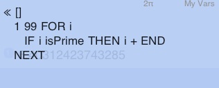
You can either type in isPrime or get it from the Integer menu. If you’re in Classic mode, the command will be ISPRIME?, which is an alias to the same function, and can be used just as well.

If you want to see more lines (10.5 to be precise)–at the cost of obscuring the soft-keys:

Your code may end with ≫ or nothing (as shown above). If you don’t add this terminating character yourself, it will be added automatically, as you enter your code.

Enter now.

You could run this code now using Eval, or store it. Let’s opt to store it, under ‘P100’.

Now tap the P100 soft-key. (We’re assuming you’re still in My Vars and showing the last page of it.)

You should get this:

Tap the ...(15 more) text.

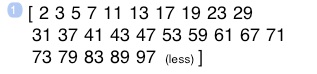
Voilà! Here’re all the primes below 100.

(If you’re getting a different result, or none at all, please double-check your code. Make sure there’s a space between “i” and “+”, etc. If you make a change, store the program again under its old name, before tapping its soft-key.)

Now, this program is pretty self-explanatory, except for two things: what’s the “[]” doing here, and how did the primes get collected in an array/list?

[] pushes an empty array on the stack. (Try entering [] on the edit line to convince yourself of that.)

Now, whenever the THEN part of the IF statement runs, i, having the value of a prime (or else we wouldn’t be in the THEN part), is added to the whatever’s on the stack, with “+”. What is on the stack? Initially, an empty list. Subsequently, the list with all previous primes added. That is, the list is “maintained” on the stack.

Finally, the program does nothing to “output” the resulting array. It doesn’t have to. The array is still on the stack, and becomes the output of the program.

This is quite terse for the task accomplished, and it demonstrates the benefit (and beauty) of balancing an item on the stack. In no more than 3 characters (“[]“ and “+”) we accomplished these tasks from the pseudo-code:

list := empty

add to list

show list

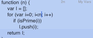
Here’s the equivalent JavaScript for the task:

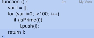
A JavaScript-specific function defined on arrays, push, is used to add i to the array.

isPrime is not part of JavaScript. It’s a function provided by MorphEngine and blended into the global namespace.

Type this in and enter, if so inclined, or skip JavaScript for the time being.

Thus far, the program produces the list of primes for a fixed, hard-coded limit: 100.

Let’s change the program so that the limit is provided by the user.

The easiest interaction with the user is to assume that he’ll put appropriate data on the stack, for the program to use as inputs. This is not only the easiest-to-implement interaction, it also permits programs to be chained with other programs, where the output of program A becomes the input of program B. (See the next section.)

Here’s how the RPL code can be adjusted to use the topmost stack item, instead of 99, as the to value of the FOR loop:

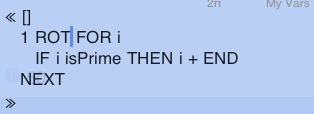
Note, “99” was replaced by ROT. ROT is a special stack operation that “rotates” items 1 thru 3 of the stack, making that the 3rd item, which, after [] and 1 were added, is the value on the stack before the program was started, becomes the 1st item again.

Enter and store this program under ‘PN’. Now, before running PN, enter a number on the stack. For example, enter 1000. Then run PN.

You should get

There’s a bunch of stack operations, such as SWAP, ROT, DUP, that are used in traditional RPL programs to manage the stack. While this can make for compact and elegant code, the approach of “balancing” items on the stack has some problems: it easily leads to code that’s hard to read and maintain. Also, it’s somewhat fragile. For example, if any other item were pushed on the stack before the ROT statement, that statement would no longer rotate in the input argument.

A way around using stack operations is to use local variables.

A better, clearer way to have an input is to rewrite the code to read:

=n assigns whatever’s on the stack to a local variable called n

This syntax is part of RPL+, and simplifies similar traditional syntax.

After assigning a local variable, you can refer to it in code, however you please. You can re-assign it at any time.

Edit the program, to adopt this new syntax.

To accommodate multiple input values, have multiple assignments to locals at the beginning of your code.

For example, if your function expects three input arguments, start your program like this:

≪ =n =beta =delta ...

Nothing forces you to use locals or assign them at the beginning of your code, but it’s good practice to do so.

Here’s the JavaScript code, adjusted to take a value from the stack as its input:

Note, all that’s changed, is that an argument has been added to the function. It doesn’t matter how the argument is named.

Multiple inputs: If you want the program to pull 3 items from the stack, add 3 arguments, etc.

Sometimes you may wish to prompt the user for a value, instead of using one from the stack. This can be accomplished with the INPUT command.

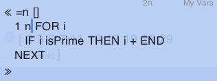
Here’s a version of the RPL program, that uses INPUT:

≪ "Prime search" "limit?" INPUT

   fromString =n

   []

   1 n FOR i

      IF i isPrime THEN i + END

   NEXT

≫

Edit the ‘PN’ accordingly and save as ‘PNinput’.

Run PNinput and you should see:

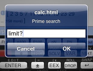
The user may now type in something and tap OK.

Their input will be returned to the program as a string.

If you want to use the input as a numerical value, it has to be converted to a number with fromString (STR→).

Getting input from a form and even live-user interface elements, will appear in version 1.5 of ND1.

Let’s say we want to find certain primes. Let’s say those, which are the square of an integer, plus one.

We could add another conditional statement to our existing code, which tests each found prime for the additional requirement of being the square of an integer, plus one, and only add those primes, which pass this additional test.

Here’s the adjusted RPL+ code, based on PN:

≪ =n

   [2]

   3 n-1 FOR i

      IF i isPrime THEN

         IF i decr sqrt isInt THEN

            i +

         END

      END

   2 STEP

≫

decr decrements by one

sqrt is √

isInt is a command that returns true for integers, and false, otherwise

There’s a new IF-conditional in the code. It says

if i decremented-by-one then-squared-rooted is an integer then add i to list endif

There’re three other changes in this code, unrelated to the newly introduced selection logic:

- 2 STEP instead of NEXT is used to increase our loop counter variable, i, by twos: 1, 3, 5, 7... That’s an optimization done in recognition that we don’t need, nor want, to test even number for primality.

- instead of an empty list, we begin with a list containing 2, the only even prime, as our new skip logic would miss it; we begin the FOR-loop with 3, the first odd number after 2

- n was replaced by n-1 because we really want to search for primes below the limit, not including it. (The to value of a FOR loop is inclusive.) n-1 would normally be written n 1 - in RPL. But RPL+ supports the given clearer syntax.

Make these edits, and store this program as ‘PNsq’ and run it:

Enter 100

Tap PNsq

You should get

So, 2, 5, 17, and 37 are primes that can be formed by squaring an integer and adding 1 to it.

Which integers would these be?

Let’s adjust the program to collect the integers instead of the primes.

In traditional RPL this is a surprisingly difficult thing to, as we’re computing the integers in question in the second IF-statement but don’t have a handle to them. Balancing them on the stack requires two statements, DUP and DROP, and use of an ELSE-branch:

≪ =n

   [1]

   3 n-1 FOR i

      IF i isPrime THEN

         IF i decr sqrt DUP isInt THEN

            +

         ELSE

            DROP

         END

      END

   2 STEP

≫

Note the lone “+”. It will add two items we’re balancing on the stack now: the array and the DUP’ed value from the second IF. This hard is hard to read.

With RPL+ you can keep the old code and structure, and simply “snapshot” the intermediate result computed in the IF, and use that snapshot where we used i before:

≪ =n

   [1]

   3 n-1 FOR i

      IF i isPrime THEN

         IF i decr sqrt =:p isInt THEN

            p +

         END

      END

   2 STEP

≫

=:p assigns a local variable; while =p consumes the item that the local variable is assigned to, =:p keeps it on the stack (hence its “snapshot” character)

This code looks a little better, but it’s not great.

Let’s store it under ‘PNsq’ and run it:

Enter 100

Enter PNsq

You should see

That is, 1, 2, 4, 6 are the integers we sought. They correspond to the primes 2, 5, 17, 37, that met our new criterion.

Sadly, looking at this code, it’s no longer obvious what it does.

Both codes suffer from one change that needed to be made: instead of starting our array with 2, the first prime, we need to start it with 1, the first integer, that after being squared and incremented, yields a prime. That is, the optimization to step in twos, is biting us here, as we’re specializing the code, further reducing readability and code maintainability.

We can do better. Enter array processing.

Let’s say we want to know the sum of the primes we’re computing.

We could adjust our program to maintain a running sum and output its final value along with the primes. (There’s nothing that prevents a function from outputting more than one result. Any number of results can be placed on the stack.)

But that would special-purpose our code and make that it harder to use it for its original purpose. If it’s changed to output two items, instead of one, a user that only wanted the primes, and not their sum, would have to drop the sum, when calling the function from another program.

It’s much “cleaner” to write a separate program that sums up elements in an array, and returns the result. Also, doing so allows use of the new program in other contexts.

Our requirements for the program are:

1. -take an array as input
   

2. -sum up all elements
   

3. -return the total sum
   

Here it is in RPL:

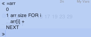
(Any name would do. Nothing identifies our input as an array.)

arr[i] is RPL+ for “element of array arr at position i ”

arr size returns the size of the array

0 is pushed on the stack, where a running sum is maintained:

the command + adds every array element to it

Enter and store this as ‘sum’.

Now, run P100, and then run sum.

You should see

We can now write a mini-RPL program like this:

Run this and you should see the same result.

Or, write

and see the same result.

Now let’s write a program that will return the sum of primes below a given number:

Think about this one for a moment. A number on the stack will become the input value to PN, which we know computes and returns an array of primes. That becomes the input to sum, which we wrote to accept an array. Its output is the final sum.

Store this program under ‘PNsum’.

Now run this on 1000 primes:

Enter 1000

Tap PNsum

You should get

Congrats on your first processing chain!

When thinking about how to sum our primes, we chose to write a separate program that computes the sum of an array. We successfully chained the two programs to yield a third: ≪ PN sum ≫

This is short and sweet and quite powerful.

ND1 has extensive array processing abilities that you can use to similar effect when developing algorithms.

Notably,

1. -any single-argument function can automatically be applied to all elements of a vector
   

2. -there’s a good number of processing functions and algorithmic patterns available, that operate on arrays
   

Often, instead of building specialization and optimization into your own code, you can leverage array processing to achieve your goal faster, with code that’s short and robust.

Picking up on what we did in the previous section, here’s how the problem can be solved with array processing:

This code, short as it is, does the same work like the last version of our program in the last section.

Store this as ‘PNsqAP’ and run:

Enter 100

Tap PNsqAP

You should see the same result as above: [1 2 4 6]

What’s happening here?

PN computes all primes.

decr decrements not just one number but *all* primes in the array that PN output

√ applies the square root to all these numbers

[isInt] filter is an algorithmic pattern that trims the elements in a given array to the ones for an associated program fragment (containing the single statement isInt here) provides a “true” condition code

This code is easy to read and, as an added bonus, runs faster than the previous code.

What if we want to go back to seeing the prime numbers, and not the generating integers?

With the previous code we needed to a real code change (and not an easy one in traditional RPL) to accomplish the switch. Now, it’s as simple as moving a bracket:

Edit the code for PNsqAP to read:

Store this as ‘PNAP’ and run it:

Enter 100

Tap PNAP

You should get again [2 5 17 37]

When manually using the calculator, you cannot “simulate” FOR-loops. You have to actually code them to see their effect. With array processing, however, you can.

You can

Enter 100

Enter PN

Tap decr (Integer menu; or just type and enter)

Tap √

Enter [isInt]

Tap filter (Array menu; or just type and enter)

That is, for certain tasks, this can help you to almost visually develop an algorithm.

Plus, you can use the record function to capture your steps into an RPL program.

When it comes to trying to writing good code, of course, nothing beats the true A and O of good software design: choosing the right algorithm. Choosing a bad algorithm will offset gains in the implementation any time.

For the last problem tackled, someone (not you) lost sight: while it might be tempting to adapt existing code to a new task at hand, the specifics may make an altogether different approach more suitable.

For finding the primes, or integers, that meet our new criterion, a forward approach is much better: instead of producing all primes and testing them for the new condition, produce all possible squares of integers, plus one, and see, if they’re primes. Since the biggest generating integer must be less than √limit, we’ll be testing a whole lot less numbers.

Here’s an efficient “forward” implementation using array processing:

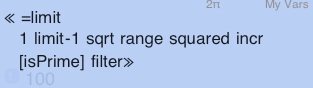
1 limit range creates an array [1..limit]

squared squares

incr increments by one

Enter this, store under ‘SPsq’, and run:

Enter 100

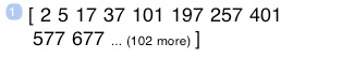
Tap SPsq

You should get the previous result of

The news is that this algorithm will gladly, and promptly, tell you the result for big numbers.

Enter 1e6

Tap SPsq

The backward approach, taken in PNsq or PNsqAP, would have to churn on this quite a while.

If, again, we want to see the generating integers, instead of the primes, a shift in the bracket does the trick:

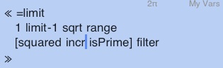
Store this under ‘SP’, and run:

Enter 1e6

Tap SP

This shows the integers known to us already, and then some.

In these implementations, note the use of range. Operating on an array/vector [1..n], is like doing all the iterations of an unconditional FOR-loop at once. So, many FOR-loops can indeed be replaced with analogous array processing.

If you’re summing something in your FOR-loop, the template 1 n range ... total will often be a better substitute.

In summary, if you need a FOR-loop you may want consider, whether array processing would work too. Conditionals are not a problems for array processing either. There’re powerful statements, like doUntil, that can even do conditional execution on a per-element basis.

Oh. It should be said: it so happens, that there’s a built-in function, primes, that does the job of PN. It employs a prime sieve (instead of testing every number for primality, as PN does), and is much faster.

If you want speed up the programs above (incl. the just named PNsq and PNsqAP), you could change PN into primes, and you should get the exact same result.

Oh2. It also so happens that there’s a built-in function, total, that does the job of sum. It, too, will make for a speedier in-place replacement.

It also so happens, that computing the sum of the primes below a certain limit, as we did above, is one of the Project Euler tasks. The complete solution to this task (#10)

surely is compact, and runs at a passable speed (39s).

The Project Euler study guide is highly recommended as a source of example programs and as a study aid. The programs are all short, but varied, and explore many ND1 programming techniques, including array processing.