Learning RPL+

RPL+ is an improved version of the RPL language found in HP calculators. It’s one of the two basic language choices you have with ND1, the other being JavaScript.

You can read this tutorial before or after Writing User Functions.

You need to know nothing about RPL or RPL+ to follow this tutorial. You are, however, assumed to be comfortable in operating the calculator in RPN mode. Knowledge of another computer programming language is helpful but not necessary. Due to its simplicity, RPL+ makes for a great first language.

This tutorial starts slow and gives examples. The focus, though, is on learning the language. There are various downloadable folders that contain RPL+ example code for you to study. Recommended are the Examples and Project Euler folders.

The good news is: If you know how to operate the calculator, you already know how to write simple RPL+ programs. That’s because, in its simplest form, an RPL+ program is a sequence of commands and data–just as you’d enter interactively into the calculator–in textual form.

There’s just one thing you also need to know:

The following is the sequence of steps performed on the calculator interactively to compute the square root of 5:

5 (enter) √

So, here’s the RPL+ program that does the same:

≪ 5 √ ≫

To enter a program, find the ≪ character and type the desired data and commands using the keypad, the iOS keyboard, and/or the soft-keys.

The edit line will not execute soft-keys when you’ve begun entering a program. Instead, it will print the function name associated with each soft-key. Likewise, the keypad will not execute functions (like √) but instead print them.

Let’s try this out.

Enter ≪ by pressing and holding the space key for a short while. (This activates the key’s 2nd function.)

Tap 5 on the keypad.

Tap the space key.

Tap √ on the keypad (press and hold the - key).

Enter.

This is how your program enters on the stack.

Note, that the ≫ closing character was automatically provided.

Your program is now on the stack at position 1, and can be subjected to commands.

You’re now ready to run the program.

Tap ⌘.

This is the result of running the program.

It’s the square root of five.

Tap the Undo (↩) key.

Let’s save the program in a variable, so we can re-use it.

Let’s use My Vars for a folder.

Check the upper right of your display to see which folder you’re in.

If it’s not My Vars, navigate there:

Tap the database (⊛) key.

Tap it again, if you don’t see a list of top-level folders, incl. My Vars.

Tap the My Vars soft-key.

Now, let’s enter the name we want for the program:

Tap the Name (‘) key (the key beneath the 2nd-level (shift) key).

Type sqrt5

Enter (this step is optional)

Tap →⊛ (Classic: STO)

The program is now stored under the name sqrt5 and you should see it among the soft-keys. (If you don’t see it, page forward using the Next Menu Page (→) key, until you do.)

To run your stored program, simply tap its soft-key.

Let’s do this now:

Tap

You will again see the result of running the program:

Let’s edit the program and make it a bit more sophisticated.

If the soft-key of a program is showing, the easiest way to recall it is to press and hold its soft-key for a short time. This will recall the contents of the key into the edit line (or the multi-line editor, as we will see shortly).

Do that now. Press and hold sqrt5 (alternatively, press the 2nd-level (shift) key and then the soft-key).

Press backspace to delete the ≫ closing character.

Tap space.

Switch to the Trig menu and tap sin.

Note, there must be a space between √ and sin.

Note, tapping sin added a space character.

You could just as well type sin. Commands inserted using the keypad or a menu will add a space character, to ready entry for the next command.

Enter.

Storing an edited version of a program is a bit simpler than storing it initially, as we don’t have to type the name. Instead, we can use the existing soft-key:

Tap the Name (‘) key.

Tap the sqrt5 soft-key.

Enter (this step is optional)

Tap →⊛ (Classic: STO)

If the name key begins an edit line, soft-keys and other commands are not run, but printed.

The edited program has been stored under the old name.

Run it, by tapping sqrt5.

The result of running the edited version of sqrt5.

This is the sine of the square root of five.

As you see, the simplest RPL+ programs are just command sequences. They’re the exact steps, you’d perform interactively.

In fact, you can use the record function from the Program menu to “write” such programs. (You did that in the Quick Tour for computing value-added tax.) You press the record button, perform your steps, and then press the stop button. The resulting RPL+ program will appear on the stack.

This method is much recommended, as you see the commands taking effect, step by step. By the time you reach the last step, you usually know that your logic and commands were correct, as you have a result to check them by.

Besides re-use, the main point of writing a program is usually to be able to apply it to varying data.

The first program we wrote, ≪ 5 √ sin ≫, is rather pointless because it only works with the number 5.

Did you notice how, in contrast, vdist worked on a new input test vector?

That’s because we started recording after entering our initial test vector. Doing so, the test vector didn’t become part of the program, and any other vector that happened to be on the stack would take its place, when the program was run again.

So, when we developed the program, we worked with certain test data, but when the time came to run it, we could provide any vector we wanted. That’s a good model to use when developing a program.

We can change the first program to also allow arbitrary input: ≪ √ sin ≫

That’s it. By taking out the 5, any number on the stack before the program is run, will now take its place.

Edit sqrt5 to look like this, and then run it on the number 10. (Which you enter on the stack, before tapping sqrt5.)

You should get this result:

This is how input works in RPL+. You simply don’t provide data in the program. Functions you use in your program that need input, will take it from the stack. The functions don’t care whether the inputs are part of the program or come from the stack.

Another way of looking at this is to consider an RPL+ program not self-contained. It’s tied to the stack, and takes what it needs from it.

And, what it leaves on the stack in excess to what it started with, happens to be the program’s “output.”

There’s no need for declaring inputs or outputs or having a “return” statement that provides output to the stack when the program is done (as is the case with most common (imperative) programming languages).

This quite simplifies working with RPL+ and is part of the reason why RPL+ programs can be very short.

Tap sqrt5 once more. You should get this result.

The result of a negative input value is a complex number.

Another neat thing about RPL+ is its automatic support for a variety of types.

The output of our program just changed to a complex number. Most common programming languages don’t support complex numbers without the help of some extra math “library”. And when they do, you have to do something special to enable support for complex numbers. In RPL+, it simply works like you’d expect.

Tap sqrt5 once more.

The result of running the program on a complex number.

Not only can the program produce complex numbers as output. It also accepts them as input.

RPL+ commands (operators, functions; these are all synonymous) usually work for a number of different data types. This is maybe the biggest strength of the language. And it, too, helps keep programs small.

At this point, it may not astonish you that your program even works for a vector of numbers.

Type 1..100

Tap sqrt5

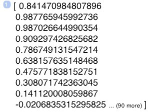
Double-tap the stack to see it full-screen.

Since the functions we used in this command chain both take and return one value, the entire program can automatically process each component of a vector, when run on one.

(You know that tapping on (90 more) will show you the rest of this 100-element result vector, right?)

Run sqrt5 one last time.

You’ll see that the result of that is now a mixed complex-real vector, with all negative elements (starting with element #10) becoming complex numbers.

Finally, let’s look at the number of inputs and outputs, taken and returnable, respectively.

Let’s write a very simple program:

Just a plus sign. Get it from the keypad.

Enter and store this as ‘plus’.

The + operator needs two inputs to operate on.

Enter 6

Enter 8

Tap the plus soft-key.

The result is unsurprising but reveals that RPL+ deals with any number of inputs. Maybe you’re starting to find that natural by now, given the description above.

Likewise, if more than one item is left on the stack when the program is done, it will have “produced” (really: left) multiple outputs.

This tutorial is about learning RPL+, the language, so we’ll not spend much more time exploring the simple command chains introduced in the last section. Let it suffice to say, that simple command sequences can already do some complex tasks. And, it helps to know the command set of the calculator well, and things like automatic array processing, to develop such chains.

As a last example of a simple command chain, let’s record the steps that solve the following problem:

We want to compute the length of an n-dimensional vector, where n can be any size.

The math formula to compute is √∑xi2, where xi are the elements of a vector x with n dimensions (or entries).

In a traditional programming language, you’d write a “for”-loop that iterates over the elements, squares them, sums them up, and compute the square root of the sum in the end.

If you know that the calculator can apply any single-valued function to an array/vector automatically, you notice that in RPL+, you won’t need a loop.

Let’s develop the solution interactively and record it.

Begin by creating a test vector of, say, 10 elements.

Type 1..10

This is short-hand notation to create a vector from 1 thru 10.

Note that this notation can also be used within a program.

Enter

Now change to the Program menu and tap the rec key. A red dot shows in the display, indicating that you’re recording.

Switch to the Real menu.

Tap x2

Any real-valued function will operate on the elements of a vector.

This is the test vector squared, component by component.

Switch to the Array menu, step 5 pages forward, and tap the total soft-key, or, perhaps easier:

Type total

Enter

The sum of all the squared components of our test vector.

Finally, dismiss the keyboard and

Tap √

The final result. The length of our 1..10 vector.

Switch back to the Program menu and

Tap stop

The three steps we performed have been recorded into one short RPL+ program.

Note, that although we dealt with and saw real data while we developed this program, none of this is recorded. Stack results are not recorded. Only the actions that are being applied. So that the resulting program will work with any data.

Store this program as ‘vdist’.

Press the database key to see the My Vars soft-keys.

Now, let’s run our program on a much larger input vector.

Type 1..1000

A vector with 1,000 components.

Tap vdist

The length of the new test vector with 1,000 elements.

This isn’t a spectacular result, but you only needed a 3-command program to achieve it. For some more explorations of command chains doing more sophisticated things, see the User Functions tutorial and Project Euler.

Now, if we really knew our command set, we’d known that there already is a function to compute the length of an n-dimensional vector.

Tap Undo (↩).

Type abs

Enter

So, a last take-away of this section is: beware of re-inventing the wheel. It pays to read the Functions reference once top to bottom, to develop a memory of what functions the calculator already has, and prevent expending time and effort on writing something that already exists.

Any programming language offers more than just execution of a sequence of commands.

Two other basic things you also want to do are:

-execute commands based on a condition
-loop

These goals are accomplished through control structures in most languages, and RPL+ is no exception. (Though it also has functions that accomplish the same goal a bit differently. We’re coming to that later.)

To conditionally execute code/steps, you employ an IF-structure:

IF condition THEN doThis END

The IF, THEN, END words in capitals are keywords. You type them exactly like this.

doThis is any number of commands

condition is any number of commands that eventually produce a boolean (true or false) or number (0 → false; not 0 → true), on which the IF structure will base its decision to execute the commands in doThis

Condition code usually compares two quantities with the <, >, <=, >=, or == operators (the equals operator == looks like this to distinguish it from the equals sign in an equation, which does not do a comparison).

Examples:

≪ IF 5 5 == THEN “five equals five” END ≫

This program compares 5 with 5 and then prints a string if it finds them to be equal. That is, if you run this program, it will print “five equals five”. The condition was true.

≪ IF 5 0 == THEN “five equals zero; wow” END ≫

This program compares 5 with zero and then prints a string if it finds them to be equal. If you run this program, nothing will print. The condition was not true.

If you want to make the comparison against an input value, remove the 5. The equals operator still needs two operands, so it will get the missing one from the stack:

≪ IF 0 == THEN “there was a zero on the stack” END ≫

If you run this program it will consume the top-most stack item, and return a string saying “there was a zero on the stack” if, and only if, that item was the number 0.

There’s an extended version of the IF-structure:

IF condition THEN doThis ELSE doThat END

It works like before but will execute the commands in doThat, if the condition is not true.

≪ IF 0 == THEN “there was a zero on the stack” ELSE “no zero” END ≫

When run, the program will now print “no zero” if the item it consumed was not a zero.

If you wanted the function to just inspect the stack, and not consume the top-most item, you’d duplicate the item before consuming it with the == operator.

≪ DUP IF 0 == THEN “there was a zero on the stack” ELSE “no zero” END ≫

(DUP is a stack command that duplicates the first stack item. It’s equivalent to pressing the Enter key when the edit line is empty. (Which is a function you’re likely to use a lot in normal operation.) You don’t need to learn stack commands if you use local variables. See the next section.)

Another thing often done in programs is to loop. That is, repeat the same code over and over.

A definite loop is called a FOR-loop in most languages. In RPL+ it looks like this:

start end FOR variable doThis NEXT

start and end are numerical values

variable is the name of a loop variable; it can be any valid variable name of your choosing

doThis is any number of commands

The loop variable will assume the values from start to end (inclusive of end), as the code in doThis is being iterated.

Examples:

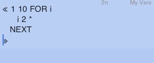
≪ 1 10 FOR i

i 2 *

You don’t have to use multiple lines and indent the doThis instructions as shown. But it’s customary and much enhances readability.

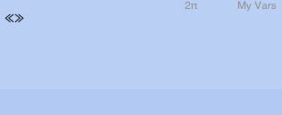
To enter this multi-line program, you need the multi-line editor. Go to the Program menu and tap the ≪≫ soft-key.

You should now see this:

You really want to use the multi-line editor for all programming.

There’re two other ways to get it:

- double-tap the edit line when no iOS keyboard is shown
- edit an existing multi-line program

The Done key on the keyboard is replaced with a return key, which will get you to the next line. The only way to dismiss the editor is to tap the Enter key.

Position your cursor between the two delimiters and begin typing the code. (Instead of positioning the cursor, you may also just delete the closing delimiter, as it will be automatically re-instated when you enter.)

Rather than typing programming keywords, you may also get them from the soft-keys in the Program menu. Page to the next menu page to see them. Only in the multi-line editor will soft-keys insert their text, rather than appending it to existing text in the edit line. If you type them, be sure to write FOR and NEXT in capitals.

Be sure to place spaces between i and 2 and * to keep these as separated commands.

It’s recommended to use 3 spaces of indentation per level.

To make visibly clear that i 2 * is the doThis block, indent it by two times 3 (=6) spaces.

Enter the program.

Tap the Eval (⌘) key to run it.

The program looped 10 times through the given commands.

Each time it pushed the current value of the loop variable i and then multiplied it by two.

The result of this is ten numbers printed to the stack. You may flick through the stack with your finger. (With ND0, you only get the first three stack positions.)

Tap Undo.

This re-instated program on the stack.

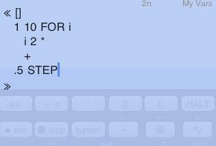
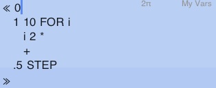
The FOR-structure also has a variation that permits you to change the increment (or step size) of the loop variable, that’s applied with each iteration.

start end FOR variable doThis increment STEP

increment is any positive or negative nonzero number

Edit the program by pressing and briefly holding the ‘ key. (This activates the key’s second function: ⇩ (Edit))

You’ll find the program back in the multi-line editor.

Super-size the editor by double-tapping it, and change the program text to read:

Super-sizing the editor gives you more room to write your program.

The downside is that it obscures the soft-keys, which are useful to speed up typing your program.

To go back to the normal size of the editor, double-tap it.

Enter this program.

Tap Eval to run it.

The iteration results are collected in an array now.

The collection in an array is due to the use of an initially empty array [] and the + operator, which, applied when an array and an item are on the stack, will add the item to the array. So the result of each “i 2 *” is added to the array.

Tap Undo, and edit this program one more time, to read like this:

Change [] into 0.

Enter and Eval.

This is the sum of the numbers that were previously added to the array.

Operators in RPL+ do many different things, depending on the inputs they’re invoked on. The + operator which was adding items to an array, is now adding the items to a running sum that’s maintained on the stack. We initialized the sum to zero before the loop.

Store this program if you want to keep it.

Whenever you think of a FOR-loop, consider the use of array processing to achieve the same result more simply.

The last three FOR-loop examples could be written (much) more simply like this:

≪ 1..10 2 * ≫

≪ 2..20 .5 * 2 * ≫ (or ≪ 2..20 ≫)

≪ 2..20 .5 * 2 * total ≫ (or ≪ 2..20 total ≫)

(total is a function found in the Array menu. It sums all elements of an array. Learn more about array processing in Writing User Functions.)

There’s another variant of a definite loop, which works like FOR but doesn’t have a loop variable:

start end START doThis NEXT

This is the simplest loop in RPL+. It will repeat the instructions in doThis end-start times.

Example:

≪ 0 1 1 10 START DUP ROT + NEXT DROP ≫

This program repeatedly adds a number to the previous two numbers on the stack. Initialized with the beginning numbers of the Fibonacci series, the programs computes the 10th Fibonacci number.

There’re two special keywords that can be used anywhere inside a START- or FOR-loop: BREAK and CONTINUE

BREAK will prematurely terminate a loop.

CONTINUE will skip the remaining code in the body of a loop and begin the next iteration.

Examples:

≪ 1 10 FOR i

IF i i * 50 > THEN “stopped at i=” i + BREAK END

This program will examine the squares of i. If i squared is greater than 50, a message will be printed and the loop will stop. This code is characteristic for a (linear) search algorithm.

Because BREAK is usually used in a conditional statement, there’s a version that combines an IF with a BREAK: IFTB (“if-then-break”). You could write i i * 50 > IFTB if you just wanted to break and not also write a message.

≪ 1 10 FOR i

IF i i * 50 < THEN CONTINUE END

i

This program, too, examines the squares of i. If i squared is lesser than 50, then nothing happens, as CONTINUE will skip the remainder of the loop body and begin the next iteration. Otherwise, i will be put on the stack. Effectively, this code will display the squares of i greater than 50. This code is characteristic for a selective processing algorithm.

CONTINUE, too, is usually used in a conditional statement, so there’s a version that combines it with an IF: IFTC (“if-then-continue”). You could write i i * 50 > IFTC instead of the IF ... END code.

Another class of loops are indefinite loops, where it’s not known a-priori how many iterations will occur. Such loops depend on a condition to become or remain true.

DO doThis UNTIL condition END

WHILE condition REPEAT doThis END

The meaning of doThis and condition is as before.

The principal difference between these two is when the condition is tested for: after first running the loop body, or beforehand.

Examples:

≪ DO

SWAP

OVER

MOD

UNTIL

DUP 0 ==

END

DROP

≫

(Credit: Patrick Dostert)

This program will execute the commands SWAP OVER MOD until the value on the stack becomes zero.

≪ WHILE

OVER

MOD

DUP

REPEAT

SWAP

END

DROP

≫

(Credit: Hideo Kogoe)

While the result of running OVER MOD DUP is nonzero, this program will execute the command SWAP.

It’s close to impossible to understand at a glance what these programs do, because they make extensive use of stack operations that are difficult for a human to read. They happen to compute the GCD (greatest common divisor) of two input numbers. You will agree they’re very elegant–if you are a stack machine.

Local variables can help make code like this much more readable.

If you have a variable stored in your local folder, you can use it in your programs. Simply refer to it by name.

For example,

enter 5

enter five

tap →⊛ (Classic: STO)

This will store the number 5 in a (global) variable, which gets a soft-key called five.

Here’s a program that uses the variable.

≪ five 2 * ≫ (to write this program, you may use the soft-key instead of typing “five”)

If you run this program, you get

Any kind of object can be stored in a variable. A number, a matrix, a screenshot, a program. If you refer to a program in another program, you “call” (execute) that program. This is just like using a built-in command/function. You pass and receive values, too, just as if you’re using/calling a built-in command/function.

In programs, you can create local variables that only exist within the program, and while it runs.

They are called local variables and, except for their limited scope and life-time, work like normal (global) variables in the calculator. That is, they are names to which you can assign any kind of object.

You create a local variable by assigning it a value using the fused = operator:

=x will assign the top stack item to a local variable called x

Note that the name of the variable is “fused” to the = sign.

Examples:

≪ 6 =six

six 2 *

≫

This program will produce the number 12.

≪ 1 10 FOR i

i 2 * =intermediate

IF intermediate 10 == THEN “found 10” BREAK END

This program will, in each iteration, assign the result of i 2 * to a local called intermediate. If intermediate is 10, it will print “found 10” and terminate the loop (via BREAK statement).

≪ 0 =sum

1 10 FOR i

i 2 *

sum + =sum

≫

This program is similar to the one from the previous section. Instead of maintaining a running sum on the stack, it uses a local variable. While this requires more code, it makes the program more readable. You immediately see that the purpose of the program is to compute a sum, and that a sum is “returned”.

sum + =sum pushes the current value of sum onto the stack, adds it to whatever’s else on the stack (here: the result of i 2 *) and re-assigns the result back to sum.

This is called incrementing a variable and is such as common operation, that there’s another fused operator for it: the =+ operator.

Here’s a shorter way to write the last program:

≪ 0 =sum

1 10 FOR i

i 2 * =+sum

≫

Note that this also works:

≪ [] =sum

1 10 FOR i

i 2 * =+sum

≫

Now, sum returns not a sum but an array of values.

If this is what you had in mind from the start, you’d probably called the local variable “arr” and not “sum”. But, incidentally, this is a useful technique for debugging: to make sure that the values you’re summing up are along expected lines, it may be useful to first inspect them in an array, and then switch over (or back) to initializing sum to zero, and producing a numerical result.

There are more fused assignment operators: =-, =*, =/

a =-x means x = x-a

a =*x means x = x*a

a =/x means x = x/a

As incrementing and decrementing by one are frequently done, there’s two operators for that: ++, --

++x means x = x+1

--x means x = x-1

Finally, you sometimes want to assign an item to a local variable and leave the item on the stack. You can accomplish this with the =: operator. It also exists together with arithmetic operations: =:+, =:-, =:*, =:/

Let’s re-write the second program above that computes the GCD, using local variables:

≪ =a =b

WHILE

a b MOD =:remainder

REPEAT

b =a

remainder =b

END

b

≫

Note:

-you can now see that this program expects two input arguments (these are assigned to locals “a” and “b”)
-you see that one result is returned, “b”
-descriptive naming of the intermediate result (“remainder”) gives a hint as to what the algorithm is doing

All three programs implement the Euclidian algorithm to find the GCD. If you know this algorithm, you probably recognized it right away in this last version.

A yet more readable version would trade

a b MOD =:remainder

for

a b MOD =remainder

remainder 0 !=

to make clear that a loop continues until the remainder of two numbers becomes zero.

Array access:

You can index into arrays using the [] operator.

To illustrate how that looks, here’s a program that runs over an array and multiplies each element by two.

≪ 1..10 =arr

1 arr size FOR i

arr[i]

2 *

=arr[i]

≫

(Array processing code for the same: ≪ 1..10 2 * ≫)

You can not only use numbers and variables for an index, but also algebraic expressions.

For example, this would be valid: arr[i*2-4*c].

Indexing defaults to “1-based”. That is, a[1] is the first element in an array called a. You can switch to “0-based” indexing by appending :0 to the index. For example: a[i:0]. You can make 0-based the default with a special command: 0[]

If you specify an index beyond the bounds of an array, it will be mapped back into the bounded range with a modulus operation. That is, you get automatic circular buffers.

An index smaller than the base index (0 or 1) will address the array from the end to the front. That is, when using 1-based addressing, 0 will address the last element. When using 0-based addressing, -1 will be the last element.

The special command any[] will disable circular buffers and allow any index to be specified. What’s more, you can use any object, such as a string, as index for an array. This converts an array into a hash-table (also called dictionary) where you associate a key with a value. Sticking to numerical indices, this creates sparse arrays.

What you can do with these is outside the scope of this introduction, but know that they exist.

You can insert comments in your program code. Type @ followed by a space character and whatever comes from there, until the end of the line, is ignored by the RPL+ processor.

Here’s an example program that shows arrays and array accessors in practice, and comments on their usage.

The program computes the number of partitions of a given integer.

≪ =n @ assign input to local “n”

0 =zero @ assign 0 to local “zero”

n mkpents =pents @ assign result of mkpents(n) to “pents”

[0 1 1 0] =signs @ assign a literal array to “signs”

[1] =partitions @ initialize an array “partitions”

0[] @ zero-based array indexing is selected

1 n FOR j

zero @ running sum

1 =k @ initialize iteration variable “k”

WHILE

j pents[k] - =:diff @ snapshot difference into local “diff”

0 >= @ compare difference (still on stack) against 0

REPEAT

partitions[diff]

signs[k] [+] [-] IFTE @ uses circular buffer “signs”

++k @ increments iteration variable

END

=partitions[j] @ assigns the next value in “partitions”

≫

Computing the number of partitions of an integer is a pretty compute-intensive task from Number Theory.

For integers beyond ~300, the 128-bit “IEEE double” data type in common CPUs (used to represent Reals in this calculator) will “overflow”, and a wrong result will be returned.

By changing the second line

0 =zero

to this

0 toBig =zero

the code above will do all math with the arbitrary-precision integer data type that exists in this calculator.

It can compute with arbitrarily large numbers, and will return the correct result for any input number.

(The “switch” to arbitrary-precision occurs because operators such as “-” will promote “normal” numbers to “big numbers” if one of the operands is a “big number”. This calculator supports both “BigInts” and “BigFloats”.)

All code examples above use RPN notation. That is, they put operands before operators:

We typed

≪ 5 √ ≫ to compute the square root of five

i 2 * to multiply i with 2

i i * 50 > to compare the square of i against 50

Mirroring the alg mode of the edit line, there’s also support for algebraic expression in RPL+.

Instead of the above, you may type

≪ √5 ≫ and

i*2 and

i*i>50

There’re two requirements:

-there must be no spaces in the algebraic expression
-if you’re using functions, they must be real-valued, or further qualified

Examples for the second requirement:

It’s ok to type sin(x) but it’s not ok to type total(arr) because total is an array function, and not a real function. You may type vector.total(arr), though.

You can mix RPN and algebraic expressions in the same program.

Using algebraic expressions can make your code more readable. For example, here’s one of the programs from above rewritten to use two algebraic expressions:

≪ 1 10 FOR i

i*2 =intermediate

IF intermediate==10 THEN “found 10” BREAK END

Often, though, RPN notation is more readable. For example, rewriting this

≪ squared total √ ≫

to this

≪ =x √vector.total(squared(x)) ≫

hardly gains readability.

In fact, RPN’s step-by-step logic is often clearer, than algebraic. Note, too, that if you use functions in algebraic expressions, you have to type parentheses and you have to provide the expected argument(s) in the form of variables or constants, as shown in the last example. You cannot rely on the stack to provide them, because the algebraic syntax demands the expression to be self-contained.

Besides these immediate algebraic expressions, there’s an algebraic expression data type.

As with any other data type, it may appear in RPL+.

For example, you could type ‘i*2’. But just like in interactive mode, entering an expression doesn’t automatically evaluate it. You have to use the @eval (EVAL) function for that.

Example: ‘i*2’ EVAL =intermediate

Just like algebraic expressions, RPL+ programs are also a data type. You can enter a program inside a program. If you do so, it will not run automatically. For that, you have to evaluate it, just like in interactive mode.

Consider:

≪ command command ≪ command command ≫ ≫

This will execute a couple of commands and then enter a program on the stack, but not do anything with it.

If you want the program to run, evaluate it:

≪ command command ≪ command command ≫ EVAL ≫

Now, not immediately executing a program, allows you to do some interesting things with it: You can pass it as an argument to commands or other programs, and you can change/manipulate it.

This mirrors powerful uses with algebraic expressions, which can be passed to functions (say draw or integrate), and which can be (symbolically) manipulated.

For example:

≪ 'x^2+5' √ sin ≫ produces the expression 'sin(sqrt(x^2+5))'

≪ 1..4 'x' peval ≫ produces the expression 'x^3+2*x^2+3*x^1+4'

When functions (programs that accept or return data) become “data”, and “higher-level” functions (programs that take functions as arguments) can be written, one speaks of a programming language being “functional”.

Thus, RPL+ is a language that’s both imperative (having sequential processing, control structures, and variables) and functional.

Before looking at some examples of what all of this means/implies, here’s one more thing to know: Commands are allowed in arrays; and strings–which can contain any text, incl. text that looks like commands–can be evaluated.

That is, both arrays and strings can become functions, too! (In addition to RPL+ programs.) While those may not use local variables, they can be quite easily manipulated. Adding operators to an array that implements a function is a process known as functional composition. Also, it opens the door to self-modifying code.

One conspicuous line of code

If you’re eagle-eyed, maybe you were wondering about this line of code in the last example of the previous section:

signs[k] [+] [-] IFTE @ uses circular buffer “signs”

Here’s what it does: the IFTE (if-then-else) function takes a condition and two arguments that will be evaluated.

In this case, the two arguments happen to be arrays that contain + and - operators. When, depending on the sign in the circular buffer, the respective array is evaluated, the + or - will be applied to whatever’s on the stack.

Effectively this line conditionally executes one command sequence or the other, depending on a condition. That’s just like an if-construct, except this is a function that excepts functions, instead of a static construct that has two (also static) branches of code.

Recursive functions

One obvious implication of function as data, is that they can be defined/created inside a program.

One use of this is to realize recursive functions (a function that calls itself) by assigning a newly-created function to a local variable and then evaluate it. Inside the function, the function calls itself by referring to the name of the local variable itself was assigned to.

Although it sounds complicated, recursive functions are sometimes the easiest way to solve a task.

This code

≪ ≪ DUP ≪ SWAP OVER MOD Euclid EVAL ≫ ≪ DROP ≫ IFTE ≫ =Euclid Euclid EVAL ≫

implements the Euclidean GCD algorithm as a recursive anonymous function. Note, how short this is in comparison to the implementations in the previous section. The code, too, uses the IFTE function but this times doesn’t take arrays but programs as “evaluables”.

Functional array processing

A number of built-in commands exist that take functions as arguments and make for quite powerful, expressive tools. Most of them operate on arrays.

Here’s a quick introduction, through examples, to some of them:

map: applies the given function to each array element

≪ 1..5 [squared] map ≫ yields [ 1 4 9 16 25 ]

Automatic array-processing makes mapping automatic for the single-valued functions such as squared (so, ≪ 1..5 squared ≫ would work all the same). But the map function allows to map any program.

fold: takes pairs of elements and successively reduces the array to a single datum, applying a binary function

≪ 1..5 [+] fold ≫ yields 15

This example would re-create the total function, which computes the sum of all array elements. If the + were changed into a * it would re-create the product function.

More complex behaviors result when the function contains more operators/commands.

This command, as well as all commands mentioned here, operates not just on numbers. Any program (that takes the right number of arguments, and returns the right number of results) can be applied to any kind of objects that it is compatible with (you can add numbers and strings and arrays, etc., but not numbers to an image...).

For example,

≪ [“this ” “is “ “a ” “sentence” [+] fold ≫ yields “this is a sentence”

filter: removes elements of an array that don’t yield true when run against a condition function

≪ 1..10 [ √ isInt ] filter ≫ yields [ 1 4 9 ]

find: returns the index of the first element in an array that passes a condition function

≪ [1 2 3 4 5 9 10] [phi 2 ==] find ≫ yields 3

select: selects the elements in one array whose indices correspond to those of a second that pass a given test

≪ [1 2 3 4 5 9 10] [1 2 1 1 2 2 1] [2 ==] select ≫ yields [2 5 9]

DOSUBS: runs a function over a variable number of elements and may yield single or multiple results of any type

≪ 1 {1 2 3 4 5} 1 [ + ] DOSUBS ≫ yields 16

doUntil: iterates a function over each element until a condition becomes true; yields final values and iteration counts

≪ [1 2 3 4 5 9 10] [phi] [1 ==] doUntil ≫ yields [1 1 1 1 1 1 1] [1 1 2 2 3 3 3]

This command has some special hints that change what it can do. The following example uses the recurse hint to iterate the function until an iteration result re-appears, that is, a cycle is detected:

≪ 105..108 [split ! total] [recurse] doUntil ≫ yields [169 169 363601 169] [12 6 8 33]

The first result array contains the final iteration results, whereas the second array indicates how many iterations it took to achieve these values.

To close, here’s a example program that does real work and utilizes a few of these commands together:

≪ 1000 primes @ generate primes under 1000

[ 100 > ] filter @dup @ filter for three-digit numbers; duplicate result

[ phi ] [ 1 == ] doUntil @ iterate the Euler totient until the result is 1

@drop2nd @ drop the result array of final values

[ 10 == ] select @ select the primes which were iterated 10x

head @ return the first number

≫

This program finds the first three-digit prime, that, when iterated with Euler’s totient function (which computes the number of co-primes of a number), yields a iteration chain length of 10.

Achieving the same with imperative constructs would require more code and be far less readable.

Functional array processing has two more benefits:

-small code changes often allow to extract other interesting results (here, for example, changing head to size would return the number of primes that generate 10-long chains; dropping the command altogether would allow one to inspect all identified primes);
-the code can be developed interactively on the calculator; you can even record it.

Both benefits conspire to make developing (and debugging) algorithms more efficient and fun.

Congratulations! You made it through another lengthy tutorial and, hopefully, learned a lot about programming ND1 in imperative and functional styles.

If you didn’t do Writing User Functions already, this would be the next tutorial to tackle. It will repeat some of what you know already but also show you new things, incl. use of the debugger and how to get input from the user.

There’s a bunch of downloadable folders available, which provide a source for plenty of example code.

If you feel like diving in and writing your own code, but rather do this on your computer with a text editor, there’re one-click (or, rather, one-tap) solutions to link your computer to ND1.