Specifications            Quick Tour            Tutorials            Reference            Forums

In this tutorial we take a look at function graphing in ND1. It is assumed that you did the Quick Tour, where you graphed an equation and interacted with it, and Just a Few More Things.

In addition to functions, or programs, which take and return one Real number as parameter, ND1 does other kinds of graphing covered elsewhere: Chart graphing is explained in Statistics, scatter plots are explained in Functions, and image drawing appears in Visualizing 987!.

Clear your stack with ⌧ (CLEAR).

Tap ∿ (PLOT) to go to the graph menu.

The function for graphing is draw (DRAW). You can tap its key in this menu to graph, or type out either “draw” (or “DRAW”) while in any menu.

Doing so will graph the “current equation”, which is found in the ‘eq’ variable of the current folder. If there’s no such variable, you get an error message.

In the Quick Tour, you were in the My Vars folder and picked up the pre-defined equation that happened to be in this folder’s ‘eq’ variable.

You inspected the current equation by tapping eq→ (RCEQ), and it looked like this

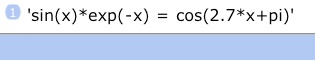
The eq→ (RCEQ) is a shorthand for recalling the ‘eq’ variable. You could accomplish the same by entering ‘eq’ and tapping ⊛→ (RCL)–that is, following the standard method for inspecting a variable. (Or, you could find it in the My Vars folder–either via the calculator’s database access key, or in My Data.)

Graphing the equation above showed two functions: one for the left, and one for the right side of the equation.

If ‘eq’ holds only one expression, opposed to an equation with an expression on either side of a “=” sign, only one function will be graphed.

Your calculator can graph various other kinds of “function” definitions in ‘eq’:

The only condition here is that each of those must take, and return, exactly one real value. The output value will be plotted against the input value in a cartesian coordinate system. (ND1 will continue to add support for coordinate systems and types of graphing in updates.)

Let’s look at the different definitions and graphing basics.

Let’s start with a clean slate:

Tap My Data and create a new folder named “Tutorial”.

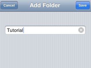
We like a new folder so we can store a new ‘eq’ variable, without overwriting one in an existing folder.

The alternative to having multiple folders when you have multiple equations you want to graph, is to name them something like ‘eq1’, ‘eq2’, ‘eq3’ and recall each in turn and store it in ‘eq’.

  Or, more simply, to store each function’s name in ‘eq’, as you will see.

Switch back to ND1 (or ND1 (Classic)) and go to the new folder:

Tap the ⊛ (USER) key twice, then tap the Tutorial key.

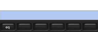
You will see a row of empty soft-keys, as there’s no data stored in this folder yet.

To explore the different function definitions available for graphing, let’s look at ways to plot the sine function.

#1 Use an expression

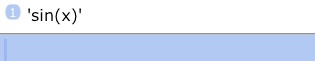
Use the Name/Expression key (‘) and type ‘sin(x

Enter.

To store this expression as variable ‘eq’ (aka “current equation”) we have two possibilities: store it like any other variable using →⊛ (STO), or use the →eq (STEQ) shorthand. For the sake of gaining practice, we’ll try both ways.

Type ‘eq

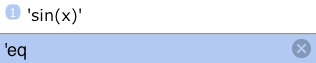
Tap →⊛ (STO)

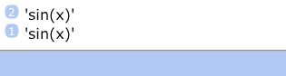
Our stack contents have been consumed and a new variable with the name ‘eq’ has been created in our new folder, which is no longer empty.

(Note, you didn’t have to tap Enter before tapping the store key.)

Tap ‘eq’ to convince yourself that it now holds our expression.

Tap ∿ (PLOT) to go to the graph menu once more.

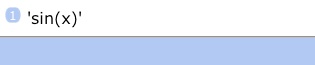
Tap eq→ (RCEQ) to recall the “current equation”.

Unsurprisingly, this returns the same expression. After all, this key is just a shorthand for recalling the current folder's ‘eq’ variable.

Tap the Drop key twice to remove the two stack items.

Tap draw (DRAW) to graph.

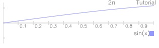
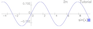
This shows the sine function in the default domain [0,1] for input values, and default range [-1,1] for output values.

Graphing domain and range are set with the minP (PMIN) and maxP (PMAX) functions. These take the coordinates of the minimum and maximum points in the coordinate system to be shown, respectively.

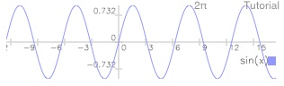
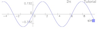
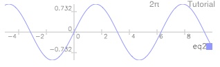
In order to see various cycles of the sine function, we have to make the domain larger. Let’s say we want to keep the range from [-1,1] but have x go from 0 to 10.

That is, our minimum coordinates remain at (0,-1), while our maximum coordinates shall be changed to (10,1).

Type (10,1 for the maximum coordinates

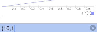
Tap maxP (PMAX)

Notice that nothing seems to have happened. What we just did is feed our new desired coordinate minimum into the minP (PMIN) function. This function registers the new point but doesn’t cause a redraw.

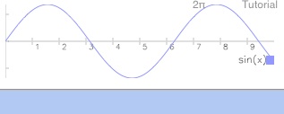
To redraw, tap draw (DRAW) again.

It’s noteworthy that minP (PMIN) is not a special function that’s only available in graphics mode. (With ND1, there’re interactive features available in graphics mode, but no graphics mode-specific functions.)

  minP is a normal calculator function that continues to work in graphics mode, like any other function.

(In case you have prior experience with HP calculators: this is a “transparent extension” of the HP calculator model.)

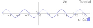
Let’s say we want to further extend the input value range: to -5, for a new minimum x value.

Type (-5,-1

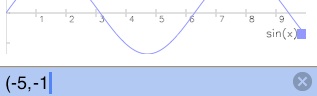
Tap Enter

Tap minP (PMIN)

Tap draw (DRAW)

(There was really no need to tap Enter. But we did it to carry home the point that the calculator continues to function normally. There’s always a stack; you just don’t see it, until you exit graphics mode.)

The next soft-key in the graphics menu is indep (INDEP). It is used to set the name of your function’s variable. If you don’t specify one, the first unknown (=undefined) variable in ‘eq’ will be assumed to be that variable. In our case that’s “x”. However, we could just as well have written ‘sin(g)’ for our expression and this would result in the same graph. In that case, ‘g’ would have been assumed to be the variable’s name. Since the variable name is determined automatically, you will rarely have a need a set it with indep (INDEP).

Just know that this function is available and that you don’t have to name our variable “x”.

Exit graphics mode, by tapping the Space key (bottom left) or the Del/Undo key. (Latter key does an undo in addition to ending graphics mode. This is mainly useful when you don’t want a displayed screenshot, or other image, which is consumed by the →screen (→LCD) function, to disappear from the stack. Tapping draw (DRAW) doesn’t consume anything, so you’re less likely to use the Del/Undo key to exit graphics mode, but it’s your choice.)

Tap My Data

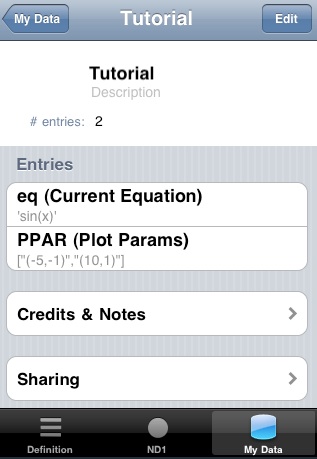
Note that there’re now two variables stored in the folder:

‘eq’, as expected (with an automatic comment that reminds you of its special meaning), and PPAR.

PPAR is the other variable with a special meaning in graphing. It contains the values for the minimum and maximum coordinate to be displayed, and, optionally the name of the variable.

If there’s no PPAR variable, default values for these two coordinates of (0,-1) and (1,1) for the minimum and maximum coordinates, respectively, are assumed.

If no variable name is present in a given PPAR variable, it will default to the first unknown variable encountered in the expression given in the Current Equation.

Switch back to ND1 or ND1 (Classic).

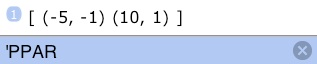
Tap PPAR

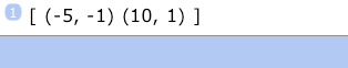
The PPAR key recalls the contents of the PPAR variable in the current folder. As you see, it contains the values we fed into minP (PMIN) and maxP (PMAX). Instead of using these functions, we could also change this vector directly. (Which can be useful when you want to set graphing parameters programmatically.)

The next two functions, *w (*W) and *h (*H), are convenience functions that operate on the coordinate pairs in PPAR. They scale the width and height of the graphing domain, and free you from having to calculate new min and max coordinates when you do scaling.

Let’s try them.

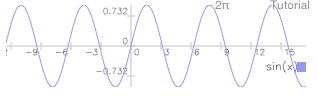
Tap draw (DRAW)

Tap 2

Tap *w

Tap draw (DRAW)

Tap 3

Tap *h

Tap draw (DRAW)

To reverse a scaling change, you use the same key with the inverse of the previous scale factor.

Type 1/3

Tap *h

Tap draw (DRAW)

In practice you will probably mostly use the pinch gesture to change the scale of your graph and to translate it. (You can try that now.)

But for exact values, or to change the aspect ratio, you’d use these, and the previous, functions that change the graphing domain and range.

Tap Space to exit graphics mode.

Our old PPAR values are still on the stack. For a case in point (and see how non-interactive manipulation of graphing parameters can be useful), store them back into PPAR:

Tap the Name/Expression key

Tap PPAR

(The Name/Expression key made that we can enter PPAR by name, versus recalling its contents.)

Tap →⊛ (STO)

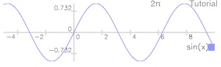
Tap draw (DRAW)

We’re back to seeing our graph within the previous coordinate system definition.

Tap Space to exit graphics mode.

Let’s get back to the various possibilities we have to define a function to graph.

#2 Use an equation

Your ‘eq’ can hold an equation, such as “sin(x) = cos(x)” and this will draw a graph for both sides of the “=” sign.

You have seen this already in the Quick Tour, so we’re not repeating it here.

If you want to graph more than two functions, just keep adding “=” signs.

For example, “sin(x) = cos(x) = tan(x)” will graph three functions.

#3 Use a function/program name

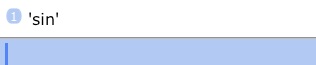
Use the Name/Expression key (‘) to type ‘sin

Tap Enter

Tap →eq (STEQ)

Tap draw (DRAW)

But you did something distinctively different: instead of graphing an expression, you graphed a function you specified by name.

Tap Space to exit graphics mode.

The name of the function can be any function or program in ND1: built-in, or user-defined in JavaScript or RPL.

Storing a function name as Current Equation yields the fastest drawing speed and also facilitates switching between multiple graphs. (See the next section.)

#4 Use a literal program

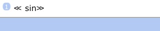
Use the RPL program key (≪) to type ≪ sin (or “≪ SIN”, if you prefer Classic)

(By the way, instead of typing “sin” or “SIN”, you can also tap the sin (SIN) key from the Trig menu.)

Tap Enter

Tap →eq (STEQ)

Tap draw (DRAW)

This time you drew a program. The program consisted of a single instruction (“sin”) but it could have been much more complex.

Any program can be used like this, as long as it takes exactly one number as parameter, and returns exactly one number as result. (HP users: this is is another “transparent extension” of the HP calculator model in ND1.)

There’s an alternative way to specify a RPL program, traditionally called “user function”: ≪ → x ≪ x sin≫≫

This kind of RPL program, too, can be used as the Current Equation for graphing.

If you want to graph multiple expressions, you have to store each in ‘eq’, one after the other, before graphing.

We recommend you keep variables like ‘eq2’, ‘eq3’, etc. in your current folder and switch to each by recalling its contents and storing it as Current Equation.

(We realize this is not as convenient as it ought to be, and will be adding a graphical UI to permit function selection in a future update.)

If you have multiple JavaScript or RPL programs, and can switch somewhat more easily by just storing the name of the function you want to graph as Current Equation, rather than its actual definition (as per method #3 above).

Here’s an example of this use:

Let’s begin by defining a JavaScript function.

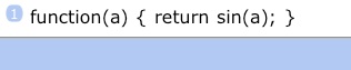
Type function(a) { return sin(a); }

Tap Enter

(By the way, if there’s a syntax error in your JavaScript function, it will not enter onto the stack. Instead you’ll be given an error message indicating in which line the error occurred.)

Type ‘eq2

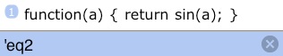
Tap →⊛ (STO)

This defined a new function in ‘eq2’.

To graph ‘eq2’ we need to make it the Current Equation.

Tap the ⊛ (USER) key.

This shows the contents of the Tutorial folder, we’re currently in.

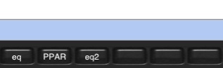
As expected there’s now a variable ‘eq2’.

Tap the Name/Expression key (‘) and eq2:

Because eq2 is a function, ND1 defaults to adding an opening parenthesis after the name. (It expects we want to write an expression that uses eq2.) In this case, we want to save some typing and obtain its name. That is, we need to remove the parenthesis.

Tap the Del/Undo key.

Tap Enter.

Tap ∿ (PLOT) to go back to the graph menu.

Tap →eq (STEQ) to store the name ‘eq2’ as Current Equation (that is, in variable ‘eq’).

Tap draw (DRAW)

Once again we’re presented with the sine graph.

This time we obtained it by graphing a JavaScript function whose name we made the Current Equation.

If we had more defined functions, we could now switch between them with relative ease, by storing the name of the function we want to graph with →eq (STEQ).

This could be done even while in graphics mode, and tapping draw (DRAW) to see the new graph.

Tap Space to exit graphics mode.

Thank you for doing the graphing tutorial! You’ve learned half a dozen ways to graph functions in your calculator, and how to numerically adjust the “window” into your graphs.